

The Fabry-Perot cavity discussed in my previous post is only a simple example of a much wider class of resonators, which control the way light behaves inside the laser and how its beam propagates outside. Each laser resonator is characterized by a refractive index function n = n(x,y,z) which may vary over space and the boundary conditions, affecting the electromagnetic field in terms of:
- spatial distribution of the electric and magnetic fields E(x,y,z) and H(x,y,z)
- resonating frequency ν
- light propagation outside the resonator, i.e. beam direction and collimation
Light propagation outside the laser cavity is possible because radiation can never be confined at 100%: such a laser would be practically useless since no beam could be extracted and used for any application.
Photonic engineering is the branch of electromagnetism encompassing the methods and techniques allowing light control by the appropriate design and fabrication of resonators.
It is an extremely wide subject, with a number of interesting theoretical, computational and experimental aspects. Photonic structures can be devised to operate in 1D, 2D or 3D, following a periodic spatial pattern or embedding defects and non-symmetric features. The huge variety of possible geometries and the use of many different materials create a wide range of applications for photonic-engineered cavities.
In order to explain the potential of such resonators, let’s consider a very narrow and thin cavity (w.r.t. the desired operation wavelength λ) which contains an active medium: this is a “wire laser“. The cavity is designed to have a sinusoidal modulation of the width along the light propagation direction (say, x-axis). Due to the narrow size of the cavity along the y-axis and z-axis, the resonator is substantially a 1D photonic system which provides a distributed feedback (DFB). The traditional mirrors of a Fabry-Perot are replaced by a structure based on a refractive index modulation spread all over the system, inducing the needed reflection and interference scheme to control light.
For example, a 10 μm-thick GaAs ridge, with an average width W = 40 μm, can be designed with a length of a few millimeters along the x-axis. It also features a sinusoidal lateral corrugation, creating a width modulation ΔW = ±10 μm with a spatial feedback periodicity Λ along the light propagation direction x (figure 6).
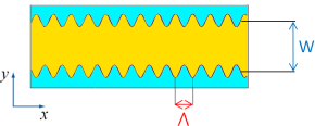
Figure 6: Sinusoidal lateral corrugation of the wire laser width W, with a spatial feedback periodicity Λ.
Indeed, changing the width of the wire laser modifies the behavior of the electromagnetic field, which is squeezed in the periodically narrower and larger cross-section of the resonator. In practice, this creates a spatial modulation of the dielectric function ε(x) for the resonating mode, having an average refractive index neff .
A first, rule-of-thumb approach to the design of such a sinusoidally modulated wire laser, requires two main information:
- the target emission frequency ν of the laser
- the expected effective refractive index neff
These are needed to set the periodicity Λ of the feedback modulation since the associated wavevector kfb needs to be properly tuned to interact with the light wavevector in the active material k = 2π neff ν/c. As shown in figure 7, light propagating in the forward direction (green arrow) needs to be back-scattered by the feedback wavevector (red arrow), so that it travels in the opposite direction along the cavity (blue arrow). This establishes the proper feedback which makes photons go back and forth across the wire laser.

Figure 7: A simple 1D model of the scattering process which makes forward propagating light (green arrow) bounce back in the opposite direction (blue arrow), due to the interaction with the wavevector associated to the feedback modulation (red arrow).
Therefore, the feedback wavevector associated with the sinusoidal width modulation has to be equal to:
and correspondingly the design feedback periodicity is:

For example, for a GaAs-based quantum cascade laser with a target operating frequency of 3.5 THz, the approximated effective index is to neff = 3.49. Consequently, a periodicity of ≈ 12.2 μm for the sinusoidal modulation provides the desired feedback for an electromagnetic mode oscillating at 3.5 THz.
PHOTONIC BAND STRUCTURE
A more complete analysis of such a wire laser requires solving Maxwell equations in a material with a 1D sinusoidal modulation of the dielectric function:

with an average value of ε0 and a modulation depth εd. Using the separation of variables, it is possible to restrict the calculation to the x-axis and consider only the z-component of the electric field (due to the polarization selection rule in quantum cascade lasers). In order to highlight its Fourier components, this function can be rewritten as:

showing that ε(x) only contains the harmonics m = -1, 0,+1. Even if the ε(x) describes an infinitely long system, it can be reduced to a much smaller portion thanks to its periodicity: a single period of length Λ. The key idea is that the electric field is itself periodic according to the geometry, i.e. E(x) = E(x+Λ), so there is no need to actually solve the problem for an infinite cavity. Therefore tools like the Bloch theorem and the Brillouin Zone reduction can be applied. In particular, the wavevectors corresponding to propagation along the x-axis are therefore limited to the reciprocal space domain k ∈ ]-π/Λ, π/Λ]. Any other wavevector outside this region can be obtained by a translation of the type k → k + m (2π/Λ) for m = ±1, ±2, ±3…
Unlike more disordered systems, all these conditions greatly simplify the solution of the electromagnetic problem which reduces to the form of the Helmholtz equation. The TM-polarized electric field (along the z-axis) can be written as a Fourier series:
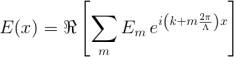
introducing the complex Fourier coefficients Em. Using the sinusoidally modulated ε(x) and the Fourier expansion of E(x), the specific Helmholtz equation can be derived:
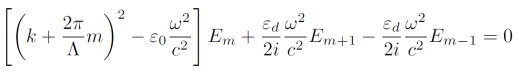
where ω = 2πν is the angular frequency of the electric field satisfying the equation. Since ε(x) only contains the harmonics m = -1, 0,+1, the resulting master equation couples each electric field component Em with the those having order m±1. The objective is using this system of equations to retrieve a formula which gives ω = 2πν of the permitted field, as a function of the wavevector k and for different orders m. A numerical solution can be implemented in a programming language such as Python or Matlab, finding for each k the corresponding frequency ν. This directly provides the dispersion relation ν = ν(k) for the sinusoidally modulated wire laser.
Before showing the numerical solution, some important physical information can be retrieved by manually solving the problem at some specific values, such as the edge of the Brillouin zone k = π/Λ for the order m = 0. In the case of a small dielectric modulation εd << ε0 and neglecting the interaction with the (m+1)-order, this perturbation approach gives two combined equations:

Based on the good old memories of linear algebra, non-trivial solutions to the above equations are those giving a system determinant equal to 0. As a result, there are two permitted angular frequencies at the Brillouin zone edge:
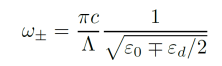
The larger angular frequency belongs to the upper band-edge mode, while the smaller frequency belongs to the lower band-edge mode. In between this two angular frequencies, no other modes are permitted so this forbidden spectral region is called “photonic bandgap”. In terms of standard frequency ν, the center frequency of the bandgap is:

which is perfectly consistent with the result obtained with the 1D wavevector scattering model. As expected from that simple representation, the target frequency is determined by the average refractive index, given by √ε0.
The difference between the upper and lower frequency gives the width of the bandgap, which is instead proportional to the dielectric modulation depth εd:

which is directly linked to the cavity width modulation ΔW. A numerical study on the propagation constant of light in a slab with width W-ΔW and W+ΔW gives an indicative value for the corresponding εd. In general, a stronger variation of the width ΔW/W induces a larger εd, producing a wider frequency bandgap.
Solving also for the spatial distribution of the electric field, the upper and lower band-edge mode have a periodicity equal to 2Λ. As shown in figure 8, the lower band-edge mode has maxima and minima in phase with the wire laser corrugation, while the upper band-edge mode has maxima and minima in counter-phase with it.
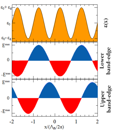
Figure 8: In the upper figure, the spatial profile of ε(x) is shown. In the central figure, the lower band-edge mode profile is plotted, for a frequency ν–. In the lower figure, the upper band-edge mode profile is shown, at a frequency ν+.
In other words, the mode at the lower frequency tends to spread covering the whole corrugation edges up to W+ΔW, while the one at the upper frequency is more concentrated in the thinner part, with a size of W-ΔW.
By considering the periodicity Λ = 12.2 μm obtained by our initial 1D wavevector-scattering model, we choose the dielectric constant ε0 = (3.49)2 = 12.18 and an oscillating contribution εd = 2.09. Following the formulae retrieved above, the bandgap center lies at νNOT ≈ 3.51 THz, while the lower frequency is ν– ≈ 3.38 THz and the upper frequency is ν+ ≈ 3.68 THz. So the bandgap width is around 300 GHz, which is 8.5% of νNOT.
Finally, the full numerical solution to the Helmholtz equation for the sinusoidal corrugation gives the dispersion relation ν = ν(k) for different orders m, producing the band structure plot reported in figure 9. The band-edge frequencies (for m=0 and k = π/Λ) are in very good agreement with the perturbation theory results shown above. 
Figure 9: The dispersion relation ν = ν (k) for different orders m is numerically computed for a sinusoidal dielectric modulation having ε0 = 12.18 and εd = 2.09.
The photonic band structure contains the complete information about the electromagnetic modes which are permitted (and forbidden) inside the corrugated wire laser, their frequency and wavevector. These modes are also characterized by the “group velocity“, which describes how fast their envelope propagates in the cavity:
![]()
Since this slope goes to zero towards the band edge, the modes around the bandgap are the slower ones. It has been shown that the slow band-edge modes are those typically more likely to lase, so the devised corrugation allows selecting the desired emission frequency.
Therefore, the emission properties of the laser can be tailored by tuning the periodicity Λ, the average cavity width W, its modulation ΔW, and carefully choosing the gain bandwidth Δg of the active material.
Of course, other aspects could also be discussed, such as the finite-size effects in a real resonator or the symmetry issues of the upper and lower band-edge modes in the far-field emission profile. Moreover, more realistic 3D models can be implemented to reproduce the physics of a resonator cavity, such as simulations based on the finite element method as explained in my post here. Since this post is just a short introduction to the methods and potential of photonic engineering, there will be time for further discussions on this blog.
Bibliography
Book by J.-M.Lourtioz, et al., “Photonic Crystals: Towards Nanoscale Photonic Devices”, Springer (2005)
PhD Thesis by the author S. Biasco (2019)
